BLS: Task Inference Beyond Least Squares in Behavioral Foundation Models

Overview

A Behavioral Foundation Model (BFM) is a single pretrained policy that can take on a new task instantly. You hand it a reward function, it turns that reward into a short task vector, and the policy conditioned on that vector is ready to run. No fine-tuning, no planning.

The catch is in how the task vector is computed. Almost every BFM uses ordinary least squares (OLS): fit the reward as well as possible on average over all states. But the states that matter most, the few high-reward ones, are usually a tiny minority. OLS happily trades accuracy on them for accuracy on the crowd of low-reward states, and the policy ends up chasing the wrong places.

BLS starts from the OLS solution and nudges it with one extra rule: keep high-reward states scored above low-reward states. This is a few hundred gradient steps on a small vector, under a second on a GPU, and it needs no environment interaction. Across navigation, manipulation, locomotion, and humanoid benchmarks, this simple change gives consistently better zero-shot policies than OLS and than prior inference methods, including ones that use online data.

Background: Zero-shot RL with Linear Rewards

A BFM represents every state and all possible tasks as vectors in a joint latent space, where their inner products define linear reward functions:

r_z(s) = \phi(s)^\top z

Here \(\phi : \mathcal{S} \to \mathbb{R}^d\) is a state feature map and \(z \in \mathbb{R}^d\) is the task vector. For each \(z\), the BFM trains a policy \(\pi_z\) by modeling its successor measure \(M^{\pi_z}(s^+ \mid s, a) = \sum_t \gamma^t \Pr(s_{t+1} = s^+ \mid s, a; \pi_z)\) and maximizing \(Q^{\pi_z}_{r_z}(s,a) = \sum_{s^+} M^{\pi_z}(s^+ \mid s,a)\,\phi(s^+)^\top z\).

At test time, given any reward function \(r\), the task vector is calculated via OLS:

\hat{z}_{\mathrm{OLS}} = \underset{z}{\mathrm{argmin}}\; \mathbb{E}_s\!\left[\lVert \phi(s)^\top z - r(s) \rVert_2^2\right]

If \(r\) lies in the span of \(\phi\), OLS reconstructs \(r\) exactly and \(\pi_{\hat{z}_{\mathrm{OLS}}}\) is optimal. In practice, downstream rewards rarely lie in this span, so the reconstruction has non-negligible errors. Crucially, OLS only cares about the total error over all states. When rewards are dense but high-reward states are sparse, OLS is pulled toward the majority of low-reward states, leaving high-value rewards poorly reconstructed and the retrieved policy suboptimal.

Our Insight: Two Sources of Suboptimality

Let \(r\) and \(\hat{r}\) be the original and reconstructed reward functions, and \(\pi_r\) and \(\pi_{\hat{r}}\) their optimal policies. The suboptimality gap is \(\mathrm{SubOpt}(r, \hat{r}) := V^{\pi_r}_r - V^{\pi_{\hat{r}}}_r\).

Theorem (Suboptimality gap)

Define the policy-averaged successor measure \(\bar{M}^{\pi}(s^+ \mid s) := \mathbb{E}_{a \sim \pi(\cdot \mid s)}[M^{\pi}(s^+ \mid s,a)]\), the successor-measure residual \(\Delta M := \bar{M}^{\pi_{\hat{r}}} - \bar{M}^{\pi_r}\), and the reward residual \(\Delta r := \hat{r} - r\). Then

\mathrm{SubOpt}(r, \hat{r}) \;\le\; \lVert \Delta M \rVert_1 \cdot \lVert \Delta r \rVert_\infty

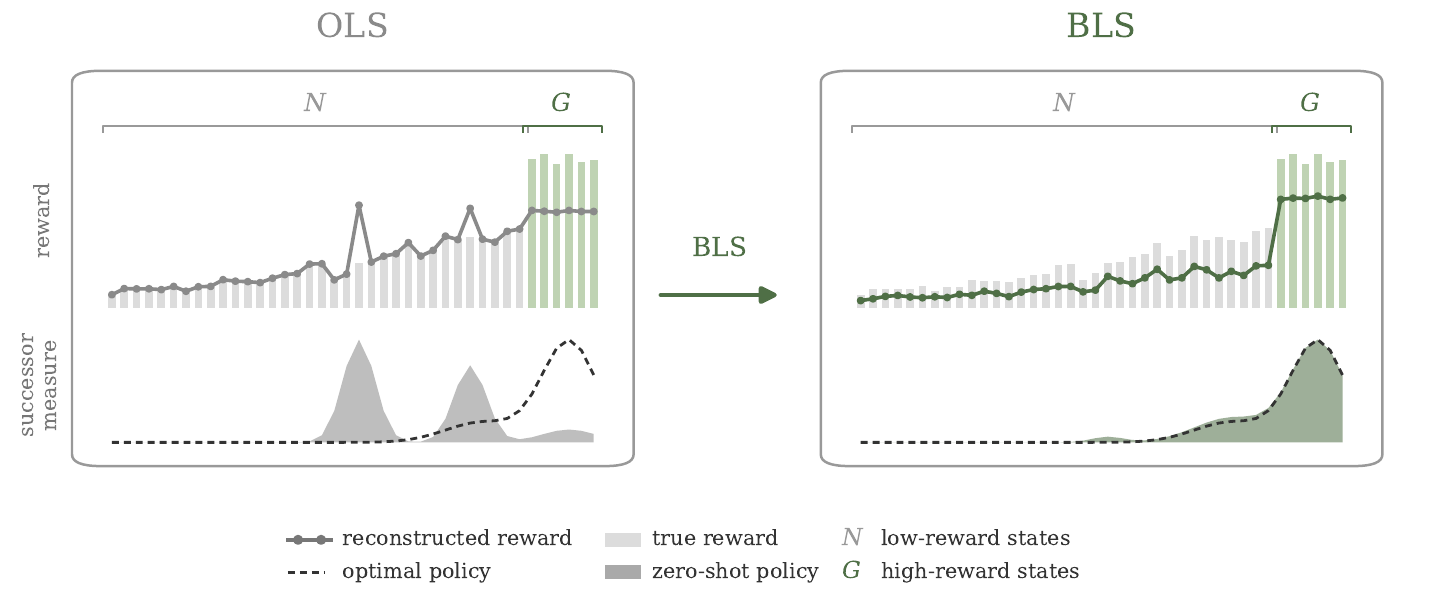
The bound vanishes under either of two conditions: the reconstructed reward matches the original (\(\Delta r = 0\)), or the retrieved policy's successor measure matches the optimal policy's (\(\Delta M = 0\)) even when rewards are wrong. OLS pursues only the first condition. Because exact reconstruction is impossible in practice, the residual rewards change the policy's behavior and enlarge \(\Delta M\). BLS seeks a task vector that minimizes both residuals jointly.

The optimal policy's successor measure is unknown at test time, so we rely on two inductive biases: (1) optimal policies visit high-reward states more often than low-reward states, and (2) reward functions sharing similar reward rankings tend to induce similar successor measures. Preserving high-value rewards and the relative ranking of rewards is therefore a practical surrogate for reducing \(\Delta M\).

Soft-margin contrastive loss

We split states into high-reward states \(G\) and low-reward states \(N\) with a threshold \(\tau\), and enlarge the margins of reconstructed rewards between the two sets:

\mathcal{L}_{sm}(z) = \log \sum_{s \in G} \exp\!\big(-\phi(s)^\top z\big) + \log \sum_{s \in N} \exp\!\big(\phi(s)^\top z\big)

The first term pushes up the lowest reconstructed rewards in \(G\); the second drives down the highest ones in \(N\). Unlike a hard-margin loss that only looks at a single worst pair, the log-sum-exp form accounts for all violating margins and is smooth for gradient descent.

Trust-region loss

The soft-margin loss alone does not control reconstruction error, so we regularize \(z\) to stay close to the OLS solution, in reward space rather than parameter space:

\mathcal{R}(z) = \mathbb{E}_s\!\left[\big\lVert \phi(s)^\top z - \phi(s)^\top \hat{z}_{\mathrm{OLS}} \big\rVert_2^2\right], \qquad \mathcal{L}(z) = \mathcal{L}_{sm}(z) + \lambda\, \mathcal{R}(z)

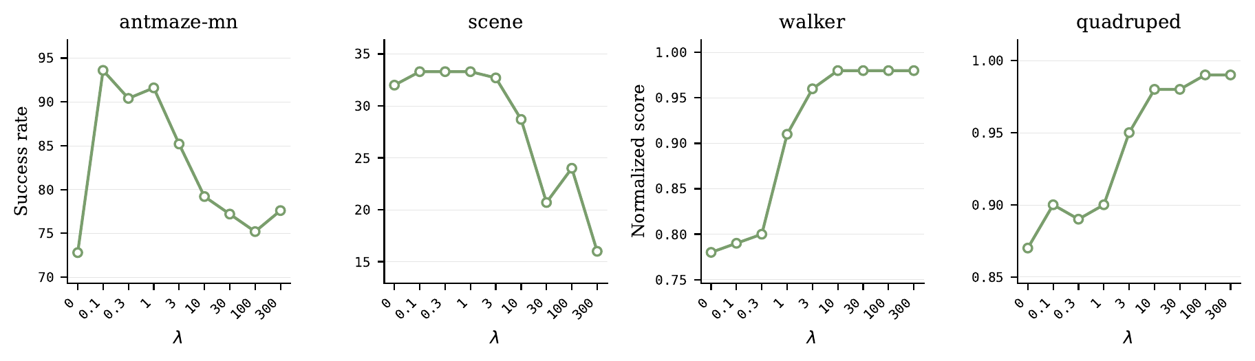
The coefficient \(\lambda\) correlates with reward type: sparse rewards prefer a small \(\lambda\) (emphasizing margins), dense rewards prefer a large one (staying near OLS).

Algorithm: BLS

Split states: \(G \gets \{s : r(s) \ge \tau\}\), \(N \gets \{s : r(s) < \tau\}\).
Initialize \(z \gets \hat{z}_{\mathrm{OLS}}\).
For \(t = 1, \ldots, T\): take a gradient step on \(\mathcal{L}_{sm}(z) + \lambda \mathcal{R}(z)\), then normalize \(z \gets z / \lVert z \rVert_2\).
Return \(z\) and retrieve the zero-shot policy \(\pi_z\).

BLS runs once before executing a task. On an RTX 4090, 500 optimization steps take under 1 second on OGBench and about 1.4 seconds on HumEnv, so the overhead relative to OLS is negligible. BLS is architecture-agnostic: it only changes how the task vector is inferred and can be plugged into any BFM, with either OLS or another inference method as the anchor.

Results

BLS Improves All Five Feature Representations

Average zero-shot success rate (%) ↑ over 9 OGBench navigation and manipulation tasks, mean over 3 seeds. The five representations are pretrained with very different objectives, yet swapping OLS for BLS improves every one of them under both observation types.

Observation	Laplacian		ICVF		HILP		FB		TD-JEPA
Observation	OLS	BLS	OLS	BLS	OLS	BLS	OLS	BLS	OLS	BLS
Proprioceptive	13.0	18.0	25.8	28.3	31.1	39.1	40.8	44.8	32.6	45.3
Pixel-based	24.5	30.3	23.2	23.3	33.4	39.4	37.5	39.1	35.7	39.8

BLS Has a Higher Success Rate than Offline and Online Baselines

Average success rate (%) ↑ on OGBench. Left: BLS is not tied to OLS. Anchoring its trust region to ZOL instead (FB representation) improves ZOL by the same margin. Right: averaged over the five representations, BLS with zero task-specific interaction outperforms ReLA and LoLA, which adapt online with 20 reward-labeled episodes per task.

OLS	ZOL	BLS@OLS	BLS@ZOL
40.8	40.2	44.8	44.3

OLS	ReLA	LoLA	BLS
28.7	20.8	27.7	35.1

BLS Has a Success Rate Comparable to Goal-conditioned RL

OGBench with HILP. Hatched segments mark the improvement of BLS over OLS. Goal-conditioned RL (GCRL) is trained directly on the goal-reaching objective and is told the goal explicitly, whereas zero-shot RL has to infer a task vector from rewards. BLS reaches 39.1% average success, comparable to GCRL at 37.7%, while OLS reaches 31.1%. Most of the gap was in the inference step, not in the pretrained model.

The Best \(\lambda\) Depends on the Reward Sparsity

Sweeping \(\lambda\) with the HILP encoder. Small \(\lambda\) means the soft-margin loss dominates; large \(\lambda\) means staying close to the OLS solution. Sparse-reward OGBench tasks (left two) gain most when the margin is enforced, and collapse as \(\lambda\) grows. Dense-reward DMC domains (right two) are already well served by OLS and prefer a large \(\lambda\). This is the failure mode from the teaser: OLS goes wrong exactly when the high-reward states are a small minority.

Task Inference Beyond Least Squaresin Behavioral Foundation Models