Learning Conditional Source Distribution
via Flow Reversal for Temporal Flow Matching

Under Review
Kuan-Hsun Tu* Hsuan-Chi Liu†* Jia-Wei Liao* Chien-Sheng Chiang Cheng-Fu Chou Tsung-Wei Ke
National Taiwan University

* Equal contribution    † Corresponding author

CNP-Flow teaser

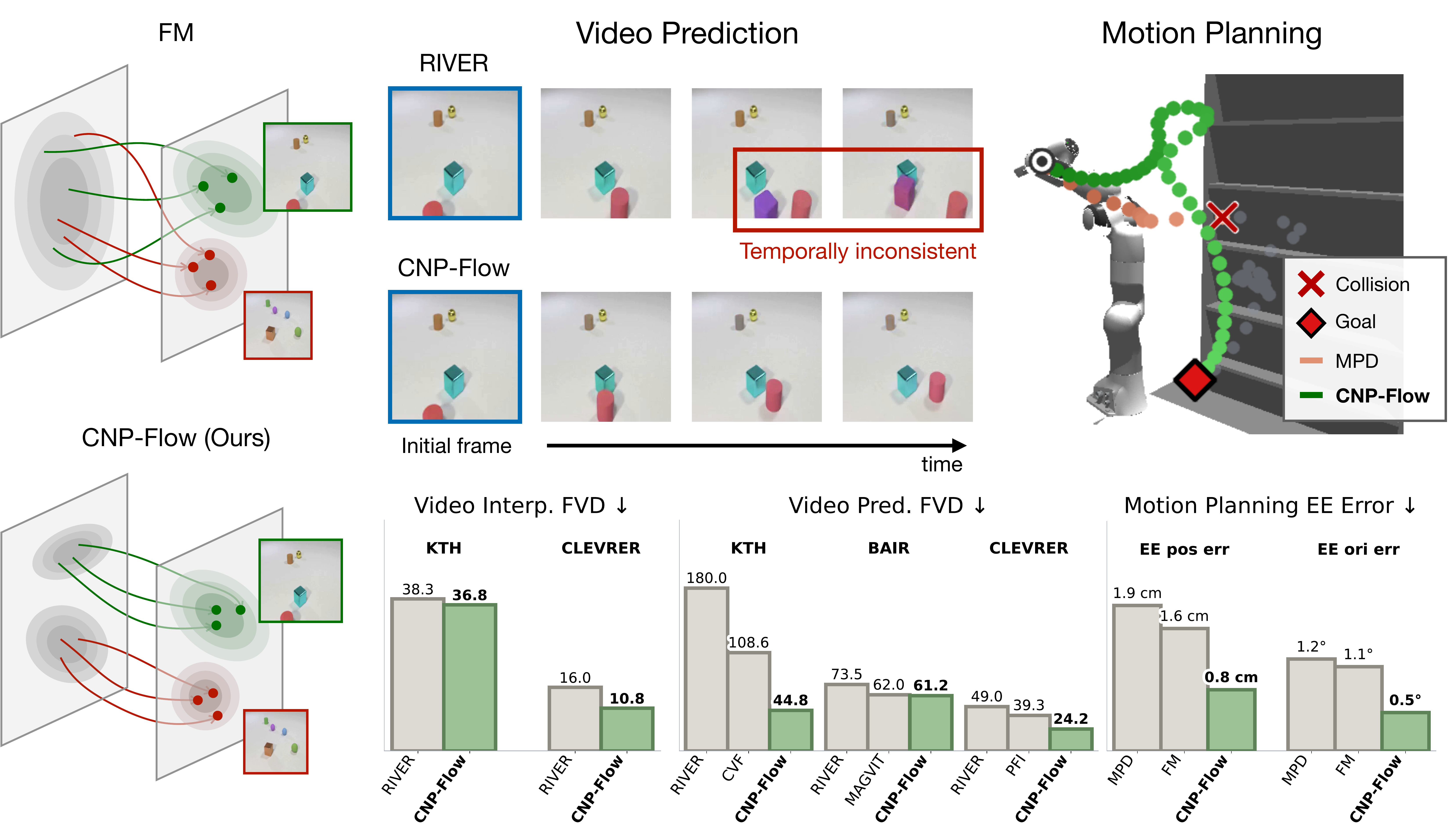
CNP-Flow learns condition-dependent source distributions for temporal generation. A Conditional Noise Predictor (CNP) predicts a source distribution for each temporal condition instead of always starting from a standard Gaussian. This source-side conditioning reduces FVD by up to 75% over RIVER on video prediction, and yields more precise motion-planning trajectories with fewer collisions.


Problem: Conditioning Only Through the Vector Field

Conditional FM trains a network \(\boldsymbol{v}_\theta\) to regress a vector field that transports a source sample \(\boldsymbol{x}_0 \sim p_0\) to a target \(\boldsymbol{x}_1 \sim p_1(\cdot \mid \mathcal{C})\), with the condition \(\mathcal{C}\) injected as an extra input:

\[ \mathcal{L}_{\mathrm{FM}}(\theta) = \mathbb{E}_{\mathcal{C},\, \boldsymbol{x}_0 \sim p_0,\, \boldsymbol{x}_1 \sim p_1(\cdot \mid \mathcal{C}),\, t} \left[\big\|\boldsymbol{v}_\theta(\boldsymbol{x}_t, t \mid \mathcal{C}) - (\boldsymbol{x}_1 - \boldsymbol{x}_0)\big\|_2^2\right], \qquad \boldsymbol{x}_t = (1-t)\boldsymbol{x}_0 + t\boldsymbol{x}_1 \]

At inference, the generated sample is obtained by integrating from a source sample:

\[ \hat{\boldsymbol{x}}_1 := \boldsymbol{x}_0 + \int_0^1 \boldsymbol{v}_\theta(\boldsymbol{x}_t, t \mid \mathcal{C})\,\mathrm{d}t \]

The output depends on both the condition \(\mathcal{C}\) and the source sample \(\boldsymbol{x}_0\). Standard FM spends all of its conditioning budget on the vector field and leaves \(\boldsymbol{x}_0\) as a condition-agnostic standard Gaussian. In temporal generation, source samples for neighboring temporal conditions can then be widely separated, and the generated sequence drifts from the target trajectory.

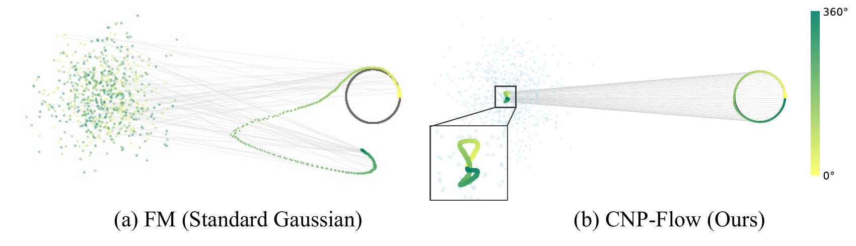
2D toy example of temporal generation

2D toy example of temporal generation. Colors indicate temporal phase along the target circular trajectory. (a) Vanilla FM draws source samples from a standard Gaussian; samples for neighboring temporal conditions can be far apart and the generated sequence deviates from the target. (b) CNP-Flow learns a conditional source with a smoother arrangement of samples by temporal phase (see the zoomed region), and the generated sequence follows the target trajectory closely.

Our Solution: Learn the Source, Keep the Backbone

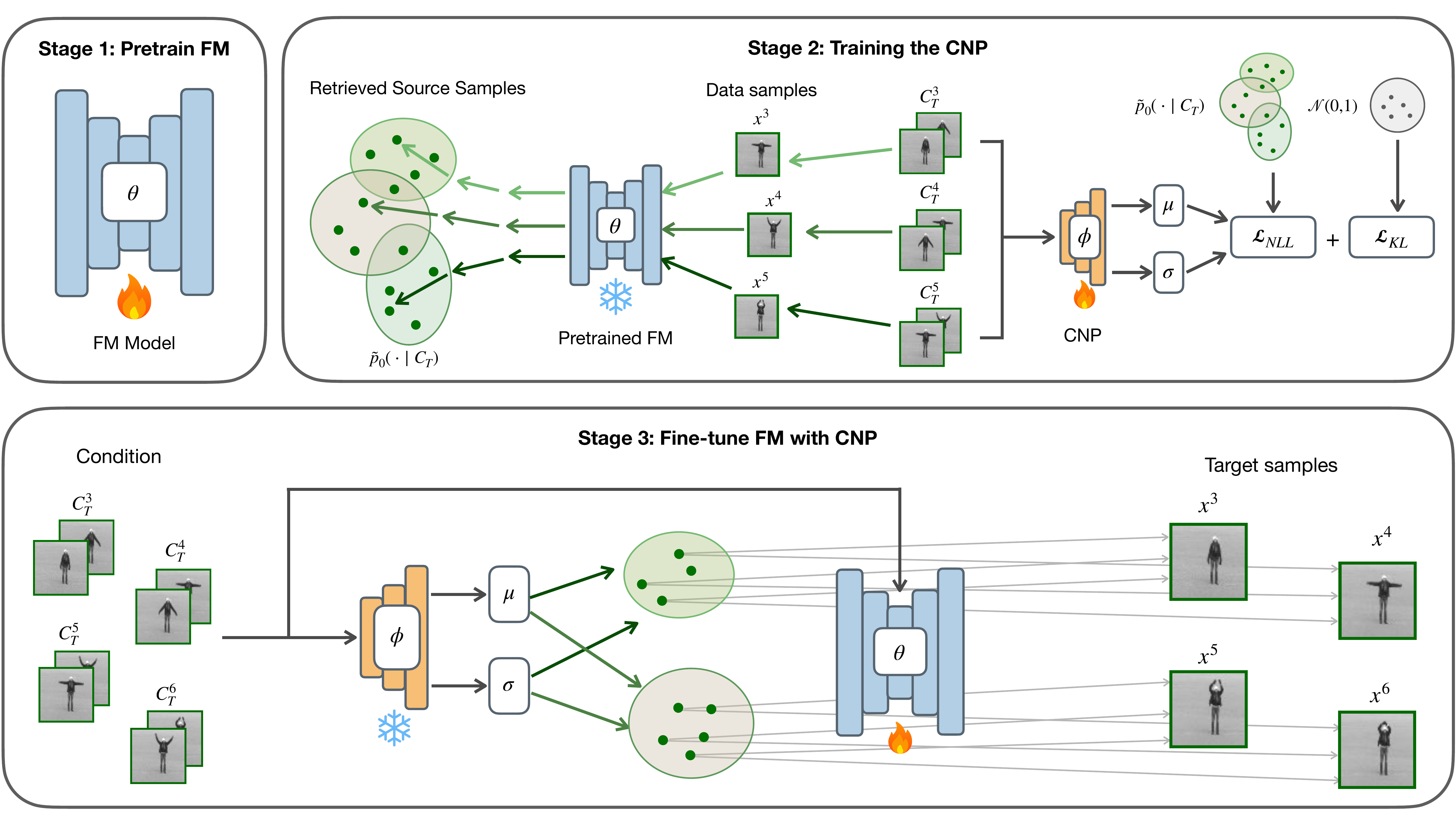
CNP-Flow three-stage training pipeline

Three-stage training pipeline. Stage 1: a pretrained FM provides flow-reversal-induced source samples that are clustered by temporal condition. Stage 2: the CNP learns to predict a conditional Gaussian prior for these samples via NLL and KL objectives. Stage 3: the FM is fine-tuned with source samples drawn from the learned prior, yielding more coherent and target-aligned transport.

CNP-Flow adds a conditional noise predictor that maps a temporal condition \(\mathcal{C}_\mathcal{T}\) to an isotropic Gaussian source distribution:

\[ p_\phi(\boldsymbol{x}_0 \mid \mathcal{C}_\mathcal{T}) := \mathcal{N}\!\left(\boldsymbol{x}_0;\; \boldsymbol{\mu}_\phi(\mathcal{C}_\mathcal{T}),\; \sigma^2_\phi(\mathcal{C}_\mathcal{T})\,\mathbf{I}\right) \]

Stage 1: Pretrain the FM, then reverse it

The FM is pretrained in the standard way with a \(\mathcal{N}(\mathbf{0}, \mathbf{I})\) source. Because the learned ODE flow is continuous, flow reversal maps nearby targets to nearby regions of source space. For each target \(\boldsymbol{x}_1 \sim p_1(\cdot \mid \mathcal{C}_\mathcal{T})\) we retrieve its source sample by integrating backward:

\[ \tilde{\boldsymbol{x}}_0 = \tilde{\Phi}_{\theta, 1 \to 0}(\boldsymbol{x}_1 \mid \mathcal{C}_\mathcal{T}) := \boldsymbol{x}_1 - \int_0^1 \boldsymbol{v}_\theta(\boldsymbol{x}_\tau, \tau \mid \mathcal{C}_\mathcal{T})\,\mathrm{d}\tau \]

This induces a per-condition source distribution \(\tilde{p}_0(\cdot \mid \mathcal{C}_\mathcal{T})\) that is clustered by temporal condition rather than spread as a standard Gaussian. It serves as the supervision signal for the CNP, sidestepping the intractable search for an optimal source.

Stage 2: Train the CNP

The CNP is trained to maximize the likelihood of the retrieved source samples, with a KL term that keeps the predicted distribution anchored to the standard Gaussian prior:

\[ \mathcal{L}_{\mathrm{CNP}}(\phi) = \underbrace{-\,\mathbb{E}_{\mathcal{C}_\mathcal{T},\, \tilde{\boldsymbol{x}}_0 \sim \tilde{p}_0(\cdot \mid \mathcal{C}_\mathcal{T})} \big[\log p_\phi(\tilde{\boldsymbol{x}}_0 \mid \mathcal{C}_\mathcal{T})\big]}_{\mathcal{L}_{\mathrm{NLL}}} \;+\; \lambda\, \underbrace{\mathcal{D}_{\mathrm{KL}}\!\big(p_\phi(\cdot \mid \mathcal{C}_\mathcal{T}) \,\|\, \mathcal{N}(\mathbf{0}, \mathbf{I})\big)}_{\mathcal{L}_{\mathrm{KL}}} \]
Proposition (Population minimizer of the NLL objective)

Over the isotropic Gaussian family, the minimizer of \(\mathcal{L}_{\mathrm{NLL}}\) has

\[ \tilde{\boldsymbol{\mu}}_0(\mathcal{C}_\mathcal{T}) = \mathbb{E}_{\boldsymbol{x}_1}\big[\tilde{\Phi}_{\theta,1\to0}(\boldsymbol{x}_1 \mid \mathcal{C}_\mathcal{T})\big], \qquad \tilde{\sigma}_0^2(\mathcal{C}_\mathcal{T}) = \tfrac{1}{d}\,\mathbb{E}_{\boldsymbol{x}_1} \big\|\tilde{\Phi}_{\theta,1\to0}(\boldsymbol{x}_1 \mid \mathcal{C}_\mathcal{T}) - \tilde{\boldsymbol{\mu}}_0\big\|_2^2 \]

The CNP's optimal mean and variance coincide with the mean and scaled second central moment of the flow-reversal-induced source distribution.

Theorem (Conditional source locality, informal)

If the predicted mean \(\boldsymbol{\mu}^*_\phi(\cdot)\) is \(L_\mu\)-Lipschitz in the temporal condition, then for two conditions \(\mathcal{C}_\mathcal{T}, \mathcal{C}'_\mathcal{T}\), independently drawn CNP source samples satisfy with high probability

\[ \|\boldsymbol{x}_0 - \boldsymbol{x}'_0\|_2 \le L_\mu \|\mathcal{C}_\mathcal{T} - \mathcal{C}'_\mathcal{T}\|_2 + \mathcal{O}\!\left(\sqrt{d\big(\sigma^{*2}_\phi(\mathcal{C}_\mathcal{T}) + \sigma^{*2}_\phi(\mathcal{C}'_\mathcal{T})\big)}\right) \]

Nearby temporal conditions yield nearby source centers; the predicted variances control the stochastic dispersion around them.

Stage 3: Fine-tune the FM with the learned source

Finally, the FM is fine-tuned with the same objective as Stage 1, but with source samples drawn from the CNP instead of the standard Gaussian:

\[ \mathcal{L}_{\mathrm{FT\text{-}FM}}(\theta) = \mathbb{E}_{\mathcal{C}_\mathcal{T},\, \boldsymbol{x}_0 \sim p_\phi(\cdot \mid \mathcal{C}_\mathcal{T}),\, \boldsymbol{x}_1 \sim p_1(\cdot \mid \mathcal{C}_\mathcal{T}),\, t} \left[\big\|\boldsymbol{v}_\theta(\boldsymbol{x}_t, t \mid \mathcal{C}_\mathcal{T}) - (\boldsymbol{x}_1 - \boldsymbol{x}_0)\big\|_2^2\right] \]

At inference, draw \(\boldsymbol{x}_0 \sim p_\phi(\cdot \mid \mathcal{C}_\mathcal{T})\) and integrate the vector field as usual. CNP-Flow only modulates the source supplied to the FM; the backbone architecture is untouched, so it drops into existing conditional FM frameworks.

One formulation, three temporal tasks

The tasks differ only in how the temporal condition is constructed:

  • Video prediction (extrapolation): at step \(i\), the previous frame is the reference and a context frame \(\boldsymbol{x}^c\) is sampled from earlier observations, \(\mathcal{C}^i_\mathcal{T} = (\boldsymbol{x}^{i-1}, \boldsymbol{x}^c, i-c)\).
  • Video interpolation: the previous frame is the reference and the final frame \(\boldsymbol{x}^N\) is a fixed future context, \(\mathcal{C}^i_\mathcal{T} = (\boldsymbol{x}^{i-1}, \boldsymbol{x}^N, N-i)\).
  • Motion planning: the whole joint-space trajectory is generated at once from the initial state and target end-effector pose, \(\mathcal{C}_\mathcal{T} = (\boldsymbol{x}^0, \boldsymbol{x}^N)\).
Results

CNP-Flow Improves Video Prediction and Interpolation with the Same Backbone

RIVER is the flow matching backbone with a standard Gaussian source. CNP-Flow keeps that backbone and swaps in the learned conditional source. \(p \rightarrow k\): \(p\) observed frames generate \(k\) future frames; \(2 \rightarrow 14\) interpolation fills 14 frames between two endpoints. CNP-Flow results are averaged over three seeds.

SettingMethodPSNR ↑SSIM ↑FVD ↓
Video prediction
BAIR64, 1 → 15RIVER——73.50
CNP-Flow20.150.83961.17
KTH, 10 → 30RIVER30.400.860180.00
CNP-Flow34.250.94344.76
KTH, 10 → 40RIVER29.000.820170.50
CNP-Flow32.690.93054.88
CLEVRER, 2 → 14RIVER——48.96
CNP-Flow42.230.99424.18
Video interpolation
KTH, 2 → 14RIVER35.650.962738.28
CNP-Flow36.070.963436.81
CLEVRER, 2 → 14RIVER43.790.994916.01
CNP-Flow45.680.995410.77

The largest gains are in prediction, where the model has to extrapolate and a good starting point matters most. Interpolation gains are smaller because the two endpoints already pin the rollout down.

CNP-Flow Also Improves Robot Motion Planning

7-DoF Franka Panda motion planning, 15 sampling steps for all methods, averaged over three seeds. Replacing the diffusion planner (MPD) with a flow model of similar size changes nothing outside noise, so the generator family is not what matters. Adding the learned source to that same flow model is what raises the fraction of valid trajectories, halves both end-effector errors, and cuts collisions by about 40%.

MethodValid (%) ↑EE pos (cm) ↓EE ori (°) ↓Collision ↓
MPD (diffusion)86.61.91.20.0030
Fixed-source FM84.91.61.10.0038
CNP-Flow (Ours)88.50.80.50.0023

The Learned Source Reduces Drift and Collisions

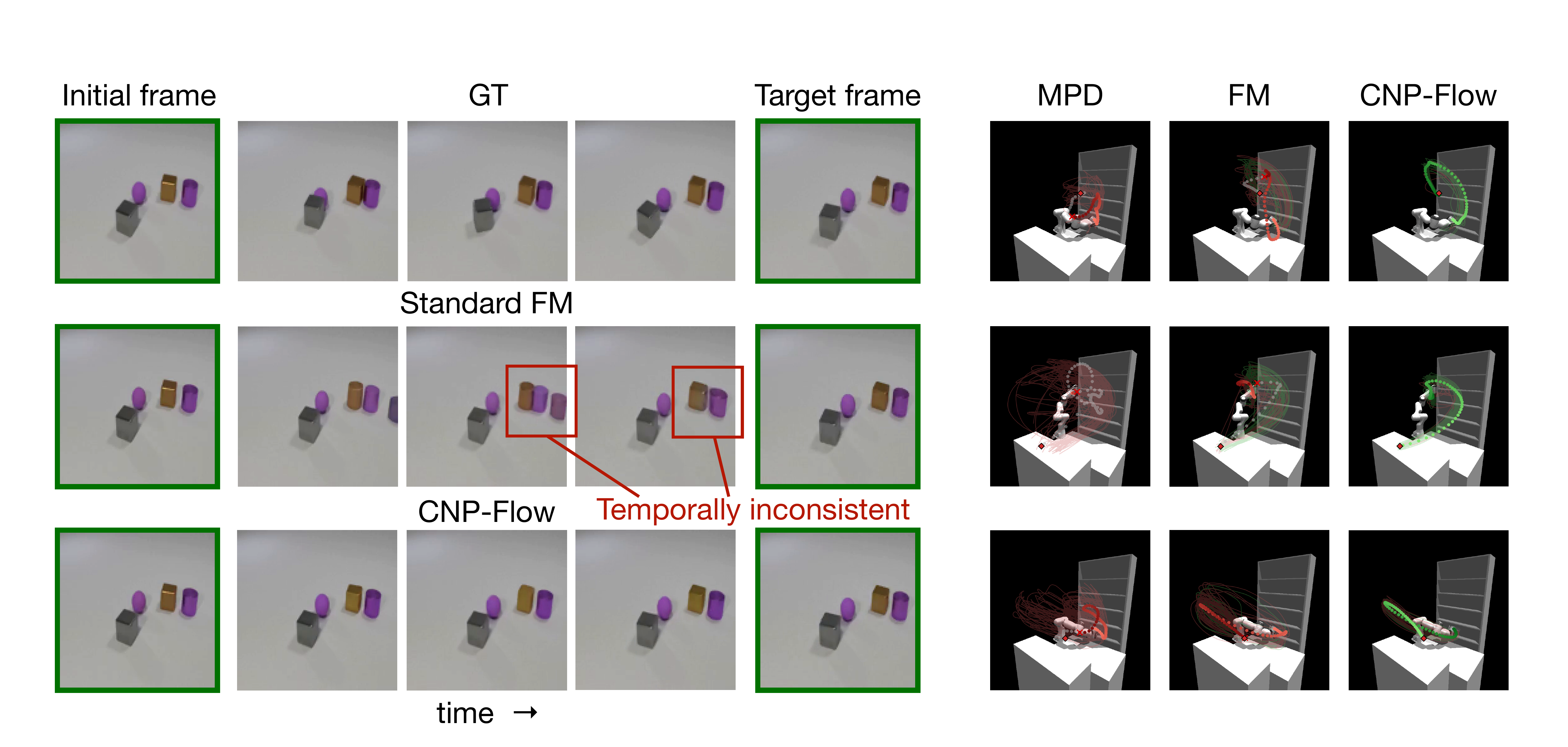
Qualitative comparison on CLEVRER and Franka Panda

Left: CLEVRER interpolation. With a fixed source the objects drift at the highlighted frames (colors fade, boundaries blur, a ghost duplicate appears), while CNP-Flow keeps object identity and tracks the ground truth. Right: Franka Panda planning, 50 sampled trajectories per panel (red: colliding, green: collision-free). CNP-Flow produces a dense bundle of valid plans where MPD and fixed-source FM mostly collide. Both failures come from the same cause: a starting point that ignores the condition.

CNP-Flow Reaches Higher Quality with Fewer Sampling Steps

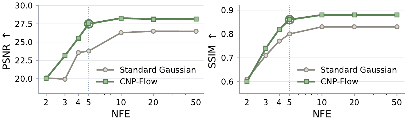
Inference efficiency on KTH prediction

KTH prediction. The plots show PSNR and SSIM against the number of function evaluations (NFE). The CNP predicts a source that is near the data manifold. Thus the ODE does not have to move samples from a standard Gaussian to the data manifold first. Each step makes a small correction. The standard Gaussian baseline reaches a PSNR of 26.5 at NFE = 10 and does not increase after that. CNP-Flow reaches a PSNR of 27.5 at NFE = 5 and 28.2 at NFE = 10. CNP-Flow at NFE = 5 has a higher PSNR than the baseline at NFE = 50.